

Fixed Income Factors: Why Do We Build Credit Curves?
Constructing fixed income factor models has long been an elusive endeavor owing to a number of challenges, not least of which includes cleansing and organizing the underlying fixed income data, or lack thereof.
Alan Langworthy
Analytics Research, SimCorp
Deciding what to model
We want to understand the composition of the total return of a bond, which includes both known and unknown returns. With this information, we can build the risk-and-return profile of a whole portfolio.
We do not need to model known returns (or carry) because this is what the holder expects to receive, unless the issuer defaults. In contrast, we do need to model unknown return and its associated risk, which depends upon price movements.
Underlying interest rates determine a significant portion of bond returns, and while this portion is greatest for higher-rated bonds, the same is still true for all but the very lowest quality credit. Indeed, many credit portfolios are managed with the duration and curve risk hedged out and a separate manager or internal desk dealing with interest rate risk. To align with the way these portfolios are managed, we separate rates from credit spread.
It is now clear what we should model: the risk and return due to changes in spread.
How should we model it?
Much of the literature on creating bond factors recommends ranking all bonds by exposure to a specified factor and bucketing them. We instead isolate individual factors through cross-sectional regression on returns. Why we do this is beyond the scope of this blog post, so here we only note that this approach requires solving.
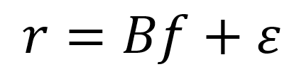
Equation 1
where r is our vector of (known) returns on a single day, B is our matrix of (known) exposures to factors, f is the vector of factor returns we seek to determine, and Ɛ is the vector of residuals we seek to minimize.
Cross-sectional regression with bond data
We could calculate returns r from spread changes or from bond returns in excess of, for instance, a duration-matched government bond or interest rate swap. With perfect or even good data, these approaches could work, although the number of bonds could still be a limitation. However, bond data is often not good: bonds mature; they have rolled prices; missing prices; and price spikes. To clean this data, we need to infer from other bonds what the spread should be.
Estimating Specific Risk
Cross-sectional regression needs only the priced bonds, not every bond on every day. For risk calculations, however, the volatility of returns usually requires an estimate of specific risk, vol(Ɛ), which requires a time series. Hence, calculating volatility of returns for new bonds is especially difficult. Instead of relying on a time series, we could set a constant volatility across all bonds, or we could assign different volatilities to investment-grade bonds and to high-yield bonds. To achieve a higher level of granularity, we bucket bonds by currency, issuer, and degree of subordination.
Tackling the Issuers
Shrinking the estimation universe reduces the hazards of using the full set of bonds, but taking a single issuer return for all securities of a given issuer and treating any differences separately seems a step too far. Equity and senior bonds from a single issuer can exhibit very low correlation as can senior and subordinated bonds, albeit to a lesser extent. A single return for each combination of issuer and subordination level is more realistic.
This single return can be achieved in several ways:
- By selecting a series of on-the-run bonds
This is harder than it sounds: the series needs to be maintained; the bonds will have varying maturities; and each bond’s maturity will shorten through time until that bond is replaced by a longer-dated one. - By creating an average return
This needs to be robust, so outliers need to be removed from a mean. We shouldn’t jump between single bonds, so taking the median return wouldn’t work. Like the previous approach, this one suffers from maturity mismatches. - By building a credit curve
With sufficient effort, we can build a robust curve from which we derive a constant-maturity bond return that overcomes many problems associated with on-the-run bonds and average returns.
The advantages of using curves
As Figure 1 illustrates, Axioma builds curves by currency, issuer, and level of subordination.
It is a return measure derived from these curves that gives us our vector of returns r in Equation 1 above. Moreover, unlike an average, a curve has shape, which we can use as we progress from modelling issuer returns to modelling bond returns.
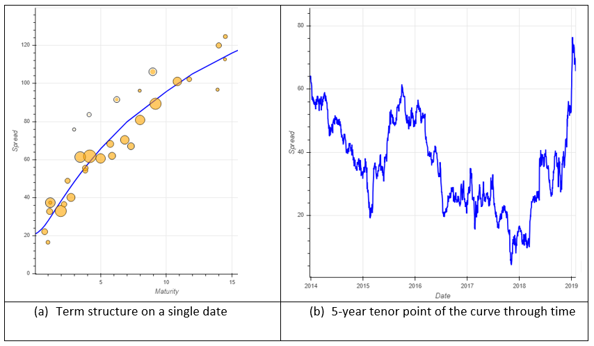
Figure 1: A credit curve built from bonds
We believe that this robust approach to building credit curves provides a more responsive model with superior back-testing and estimation capabilities. In development for several years, our proprietary methodology solves for the main challenges inherent in other fixed income risk models.
Related articles