5 ways factor-mimicking portfolios reveal hidden insights

Whether by design or circumstance, every portfolio either invests or hedges factors with direct consequences for risk and return. Factor-aware portfolio managers routinely consider exposures to factors, alongside their return, volatility and correlation trends, resulting in better outcomes for realised portfolio return and risk.

So what’s the problem? 

This approach overlooks a crucial dimension: Factors, just like portfolios, have characteristics that go beyond return and volatility. A manager would never invest in a portfolio without awareness of its turnover, concentration and underlying structure so why ignore this broader perspective?  

Historical return trends, volatilities and factor definitions give good ‘macro-intuition’ for each factor, but ultimately factors are constructed bottom-up from assets and have a direct representation as a portfolio – a factor-mimicking portfolio (‘FMP’).

What are Factor-Mimicking Portfolios?  

In cross-sectional factor models, FMPs are a mathematical by-product of the regression. Each FMP has one-standard-deviation exposure to its own factor and zero exposure to any other risk factor – the purest representation of a factor possible . FMPs track their respective factors’ performance and risks, but are unconstrained by transaction costs and turnover when the model is re-estimated – typically daily.

Despite this, FMPs are the definitive representation of their factors and can help practitioners understand factor behavior. Here, we explore five practical applications.

1.    Gaining factor stability intuition with concentration and turnover

‘Value’ and ‘Fundamental’ – factor types relying on low frequency financial statement data – have the lowest turnovers, indicating these types of factors are relatively more stable. Meanwhile, technical factors, especially those with shorter lookbacks like Short-Term Momentum (STM) show higher turnovers. Notably, Size, Downside Risk and Residual Volatility are comparable to STM. Meanwhile, Opinion Divergence, which measures relationships between traded volumes and returns is transient, therefore unrealistic to hedge.

Figure 1: Average Turnover by Style Factors 

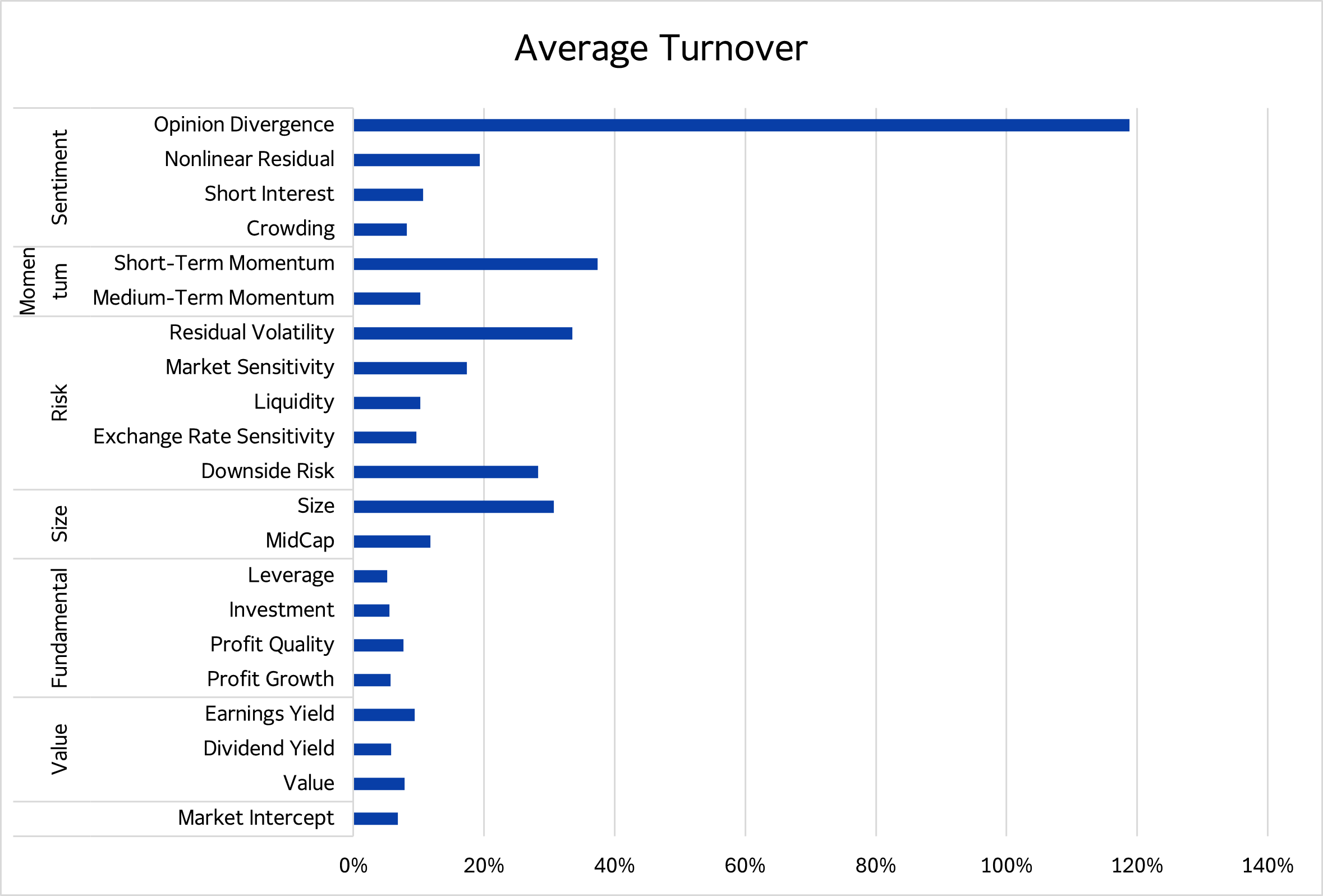
Source: Axioma US Equity Factor Risk Model (v5.1) 

FMPs are diversified because of minimized residual returns, so concentrations are low. But Size, a skewed distribution with mega cap concentration and Market Intercept, the only net long FMP, have effective names counts of 300 or less, indicating elevated concentration compared with other factors.

Figure 2: Average Effective Number of Names

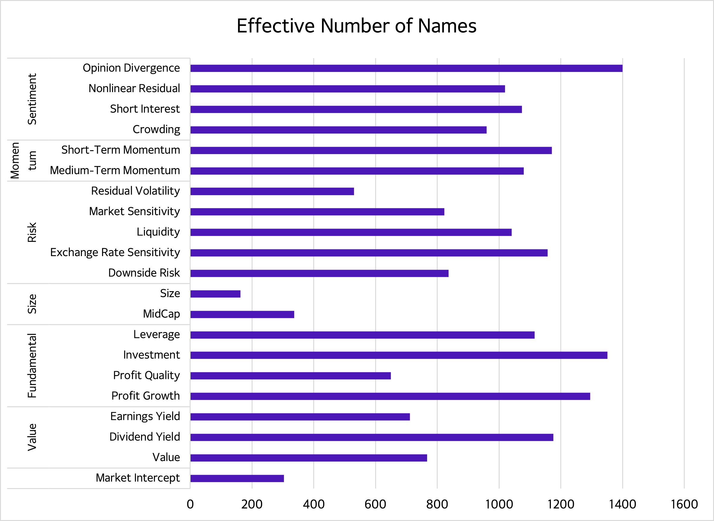
Source: Axioma US Equity Factor Risk Model (v5.1). Effective Number of Names is the reciprocal of the sum of the squares of the portfolio weights. Monitoring these metrics over time can reveal important regime shifts and FMPs can make those shifts much more obvious.

2. Serving as an early warning system

While traditional factor returns rely on end-of day returns, FMPs can be monitored intraday. This use case requires the FMP to ignore prior day (realized) asset returns and incorporate the latest possible exposures data as a regression input . This way, factor performance can be monitored as it happens, and significant moves can be used as an early warning system to anticipate where the factor is heading, before it is published.

3. Revealing structure within factors through return attribution

The return sources within FMPs can be analyzed by decomposition into traditional groupings, for example by sector, market cap or the long/short legs. The Crowding factor illustrates the latter. Returns occur almost entirely on the long leg with the short leg hedging the impurities on the long side. This insight has implications for portfolio construction: it suggests that neutralizing this factor is best done by underweighting names on the FMP long leg, rather than overweighting names on the FMP short leg. Furthermore, although the pure factor return (13.4% cumulative) is strong, the long leg impurities (especially Size, Short Interest, Profit Quality) drive an overall negative performance on the long leg. Therefore, to take a pure positive exposure on the factor, offsetting other exposures is critical. 

Figure 3: Return Attributions

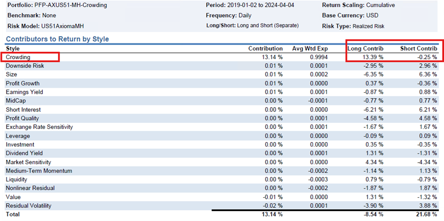
Source: Axioma Portfolio Analytics

 4.    Measuring the impact of factors across models 

Factors are pure in the context of their own model but may show relationships when viewed through the lens of a different factor model.

Below, a secondary model is used to attribute the returns of a Profit Quality FMP (blue). Most of the return is understood by the second model’s own Profitability factor (yellow) but a significant portion is unexplained asset-specific return (purple). This occurs because the profitability factors in each model have significant overlap. They share descriptors, but the Profit Quality factor includes new ones (Gross Profit to Assets, Accruals to Assets, Sales to Enterprise Value) that are not perceived as systematic risk in the second model.

This type of analysis can give comfort about the impact of factor definition changes, and importantly, it can help measure the incremental effect of new descriptors.

Figure 4: Profit Quality Returns Attribution Across Models

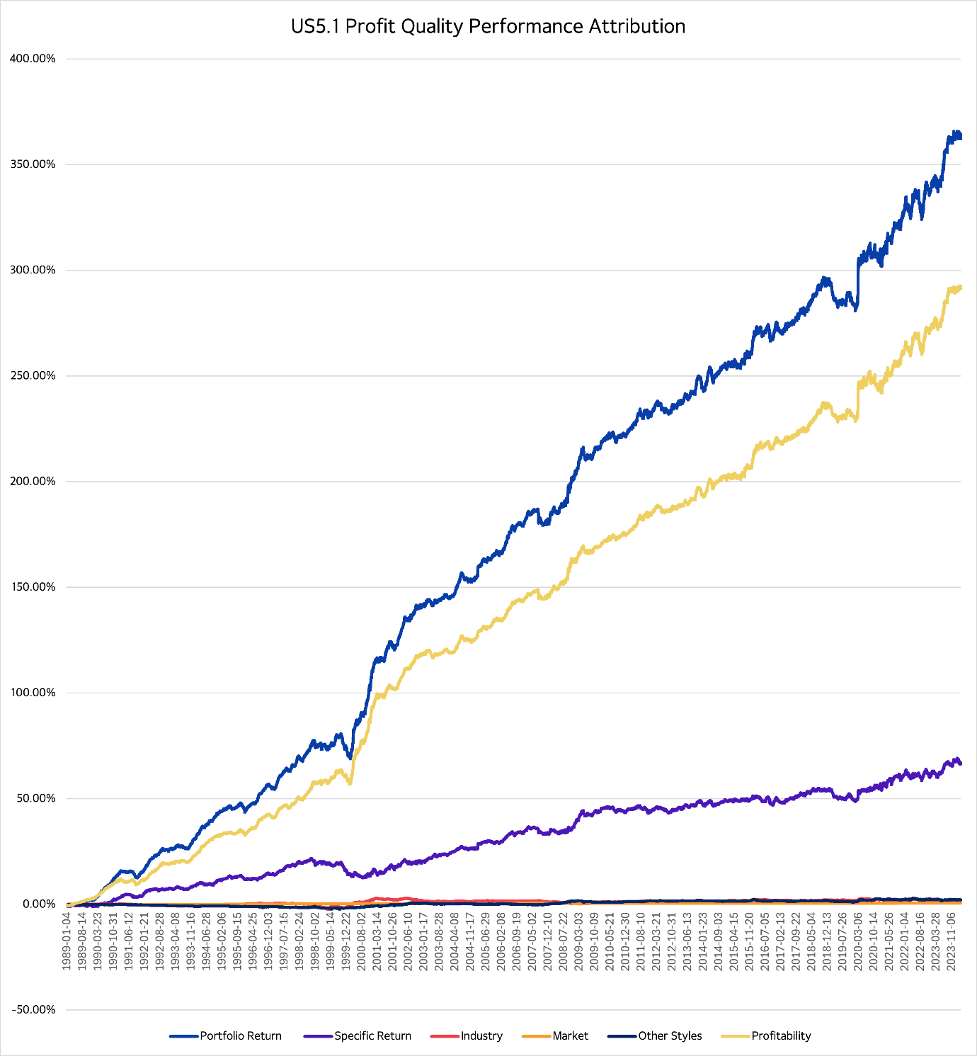
Source: Axioma Portfolio Analytics, Axioma US Equity Factor Model (US5.1)

5.    Implementing more realistic factor strategies 

You can’t invest in an FMP directly, but if you wanted to invest or hedge a factor, you still are approximating it, subject to tradability and other criteria. By understanding the replicability – how closely factor returns can be matched – alongside turnover, more cost efficient and/or more balanced approaches to factor-based portfolio construction emerge. For example:

• Minimizing tracking error to the FMP
• Rebuilding the FMP, allowing impurities 
   

Each of these possibilities could be framed with or without complementarity to an existing portfolio and/or a benchmark .

Unleashing the full potential of factor analysis 

Factor-mimicking portfolios (FMPs) provide a mathematically rigorous representation of factors often underutilized by practitioners. They enable portfolio managers to evaluate factors like portfolios, beyond just risk and return. This approach leads to better factor understanding and more holistic investment decisions. Contact us to learn more.

1. In a linear cross-sectional factor model, asset returns r are expressed as exposures X onto factor returns f, plus a residual u with the equation r=Xf+u . The weighted least squares solution is f=(X^T WX)^(-1) X^T Wr, which maps factor returns directly back to asset returns, the transition matrix.(X^T WX)^(-1) X^T W implicitly contains the factor mimicking portfolio weights.

2. Email [email protected] for a more detailed explanation.

3. See ‘What, Exactly, Is a Factor?’ to see this in practice.